Dimensionar una batería de arena para 17 viviendas españolas
Notebook · 2026
El capítulo 4 de un trabajo de ENGF0004, reconstruido como modelo ejecutable —cada cálculo a mano se convierte en una función y cada resultado se contrasta con la cifra publicada en el informe.
Funciona en Colab sin instalar nada: solo numpy y matplotlib. Cada resultado se contrasta con la cifra que recoge el informe original.
Batería de arena — propuesta de diseño
Un almacén térmico estacional para 17 viviendas españolas, hecho con residuos reciclados de baldosa cerámica.
Este notebook reproduce el capítulo 4 (Propuesta de diseño) de ENGF0004 Coursework 2 como código ejecutable: cada hipótesis se convierte en una constante con nombre, cada cálculo a mano en una función, y cada resultado se contrasta con la cifra publicada en el informe.
¿Para qué molestarse, si el informe ya tiene los números? Porque una hoja de cálculo de un diseño te dice lo que cuesta ese diseño. Un modelo parametrizado te dice sobre qué hipótesis se sostiene el diseño —y en este sistema la respuesta resulta ser un único número que nadie midió.
El problema
Se prevé que España alcance 39 GW de fotovoltaica en 2030. Eso crea una curva de pato: la generación tiene su pico a mediodía, la demanda residencial por la tarde-noche, y el desfase llega a unos 20 GW a lo largo de una franja de 5 horas por la tarde. Si no hay dónde meter el excedente, se recorta: se genera y se tira.
Una batería de arena es una de las respuestas menos glamurosas que existen. Se calienta un montón de sólido granular barato con la electricidad sobrante, se aísla y se le hace pasar aire cuando se necesita recuperar el calor. Sin litio, sin química de degradación, sin cadena de suministro. La pregunta de ingeniería es siempre la misma: ¿cómo de grande tiene que ser el montón y qué falla primero?
Preparación
Aquí no hay que instalar nada en Colab: numpy y matplotlib vienen incluidos.
import numpy as np
import matplotlib.pyplot as plt
from matplotlib.ticker import FuncFormatter

# One place to change the look of every figure in the notebook.
PALETTE = {
    "accent":   "#2a78d6",
    "accent_2": "#7db3ea",
    "warn":     "#c2564d",
    "ink":      "#1b1b1b",
    "faint":    "#8a8a8a",
    "grid":     "#d8dce4",
}

plt.rcParams.update({
    "figure.figsize":   (8, 4.5),
    "figure.dpi":       120,
    "font.size":        11,
    "axes.grid":        True,
    "axes.axisbelow":   True,
    "grid.color":       PALETTE["grid"],
    "grid.linewidth":   0.8,
    "axes.spines.top":   False,
    "axes.spines.right": False,
    "axes.edgecolor":   PALETTE["faint"],
    "axes.titlesize":   12,
    "axes.titleweight": "semibold",
})

def check(label, computed, reported, tol=0.01, unit=""):
    '''Compare a computed value against the figure printed in the report.

    tol is a RELATIVE tolerance, because the report rounds as it goes. A mismatch
    is printed rather than raised: some of them are informative rather than wrong.
    '''
    rel = abs(computed - reported) / abs(reported) if reported else float("inf")
    ok = rel <= tol
    # Kept under 72 columns so it reads on a phone as well as in Colab.
    print(f"{'ok ' if ok else 'DIFF'} {label:<30} {computed:>12,.1f} vs "
          f"{reported:>12,.1f} {unit:<6} {rel*100:5.2f}%")
    return ok

print("Ready.")
Ready.
4.1 Hipótesis y parámetros elegidos
Cada número de abajo es una elección de diseño con una fuente detrás. Están reunidos aquí para que el resto del notebook no tenga constantes ocultas: si quieres rediseñar la batería para otro clima u otro parque de viviendas, esta es la única celda que hay que editar.
El parque de viviendas
| Hipótesis | Valor | Por qué |
|---|---|---|
| Viviendas atendidas | 17 | El tamaño medio de una promoción residencial española, estable desde mediados de los noventa |
| Calificación energética | Letra E | La calificación más común en España: el 55,9 % del parque |
| Consumo específico | 190 kWh/m²/año | Estimación central de la horquilla 151–230 de la letra E |
| Fracción para calefacción | 63,9 % | |
| Fracción para agua caliente | 10,7 % | |
| Superficie de la vivienda | 186,7 m² | Media española de vivienda unifamiliar |
| Fracción útil | 85 % | Excluye escaleras exteriores y garajes, que no se calefactan |
| Temporada de calefacción | 182 días | Del 15 de octubre al 15 de abril |
| Días de autonomía | 2 | Aproximadamente la mitad de los días de enero están nublados en el centro de España |
# ---- Housing stock ----------------------------------------------------------
N_HOUSES            = 17
SPECIFIC_KWH_M2_YR  = 190.0     # kWh/m2/yr, band E central estimate
FRAC_HEATING        = 0.639
FRAC_HOT_WATER      = 0.107
FLOOR_AREA_M2       = 186.7     # m2, average Spanish single-family home
USABLE_FRACTION     = 0.85      # excludes stairs and garage
HEATING_SEASON_DAYS = 182       # 15 Oct - 15 Apr
DAYS_PER_YEAR       = 365
AUTONOMY_DAYS       = 2

heated_area = FLOOR_AREA_M2 * USABLE_FRACTION
print(f"Heated floor area per house: {heated_area:.1f} m2")
check("heated area", heated_area, 159.0, tol=0.01, unit="m2")
Heated floor area per house: 158.7 m2
ok  heated area                           158.7 vs        159.0 m2      0.19%
El medio de almacenamiento
El informe sustituye la arena por residuos reciclados de baldosa cerámica triturada, por tres motivos:
- Aproximadamente el doble de capacidad calorífica volumétrica que la arena seca (2,4–3,4 frente a 1,3–1,6 MJ/m³/K), lo que reduce directamente el tamaño de la batería.
- Es químicamente estable a alta temperatura, así que el rango de operación puede ser más amplio.
- España es uno de los mayores exportadores mundiales de baldosa cerámica: la materia prima es un subproducto industrial, no un material que haya que comprar.
Un lecho granular no es macizo. Solo la cerámica almacena calor; los huecos son aire. La fracción de empaquetamiento aparente es la parte del recipiente que ocupa realmente el sólido, y se toma para esferas empaquetadas al azar:
# ---- Storage medium: recycled ceramic waste ---------------------------------
RHO_S          = 1900.0     # kg/m3, bulk density (range 1,730-2,050)
CP_S           = 1526.0     # J/kg/K, derived specific heat capacity
K_S_RANGE      = (0.33, 1.01)  # W/m/K, thermal conductivity - LOW, see 4.3
PACKING_PHI    = 0.60       # randomly packed spheres

rho_eff = PACKING_PHI * RHO_S
cp_eff  = PACKING_PHI * CP_S

print(f"Effective density          rho_eff = {rho_eff:,.0f} kg/m3")
print(f"Effective specific heat    cp_eff  = {cp_eff:,.0f} J/kg/K")
check("effective density",      rho_eff, 1140.0, unit="kg/m3")
check("effective specific heat", cp_eff,  916.0, unit="J/kg/K")
Effective density          rho_eff = 1,140 kg/m3
Effective specific heat    cp_eff  = 916 J/kg/K
ok  effective density                   1,140.0 vs      1,140.0 kg/m3   0.00%
ok  effective specific heat               915.6 vs        916.0 J/kg/K  0.04%
Rango de temperaturas de operación
con la carga completa, una vez agotada, así que .
El límite superior es un límite de materiales: la cerámica reciclada se ensayó hasta 610 °C sin agrietarse durante más de 60 ciclos, y los almacenes comerciales de arena llegan a 600 °C.
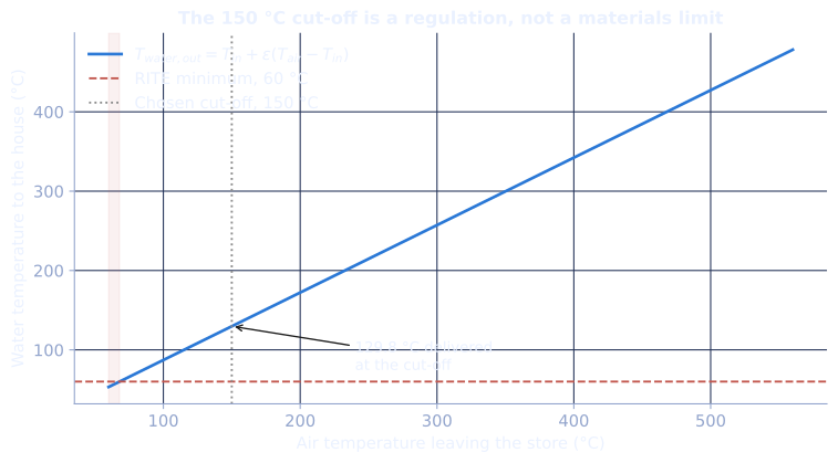
El límite inferior no es un límite de materiales: es normativo. El RITE español dimensiona los circuitos de radiadores para una impulsión/retorno de 60/40 °C, así que el intercambiador tiene que entregar agua a 60 °C o más. Con la relación -NTU de un intercambiador a contracorriente:
# ---- Operating range and air/water exchanger --------------------------------
T_HOT          = 550.0      # degC, fully charged
T_COLD         = 150.0      # degC, fully discharged
DELTA_T        = T_HOT - T_COLD
CP_AIR         = 1050.0     # J/kg/K, evaluated at the 350 degC mean
EPSILON_HX     = 0.85       # counterflow heat exchanger effectiveness
T_WATER_IN     = 15.0       # degC, ground water at 15 m depth
T_WATER_REQ    = 60.0       # degC, RITE minimum flow temperature

def water_outlet(t_air_in, t_water_in=T_WATER_IN, eps=EPSILON_HX):
    '''epsilon-NTU outlet temperature for the domestic circuit.'''
    return t_water_in + eps * (t_air_in - t_water_in)

t_out_at_cutoff = water_outlet(T_COLD)
print(f"Delta T across the store: {DELTA_T:.0f} degC")
print(f"Water delivered at the {T_COLD:.0f} degC cut-off: {t_out_at_cutoff:.2f} degC"
      f"  (RITE needs {T_WATER_REQ:.0f})")
check("water outlet at cut-off", t_out_at_cutoff, 129.75, unit="degC")

# The cut-off could in principle go lower. Where does it actually bite?
t_air_min = T_WATER_IN + (T_WATER_REQ - T_WATER_IN) / EPSILON_HX
print(f"\nAir temperature at which the circuit JUST reaches 60 degC: {t_air_min:.1f} degC")
print(f"Chosen cut-off sits {T_COLD - t_air_min:.1f} degC above that — a deliberate margin.")
Delta T across the store: 400 degC
Water delivered at the 150 degC cut-off: 129.75 degC  (RITE needs 60)
ok  water outlet at cut-off               129.8 vs        129.8 degC    0.00%

Air temperature at which the circuit JUST reaches 60 degC: 67.9 degC
Chosen cut-off sits 82.1 degC above that — a deliberate margin.
air_in = np.linspace(60, 560, 400)
w_out  = water_outlet(air_in)

fig, ax = plt.subplots()
ax.plot(air_in, w_out, color=PALETTE["accent"], lw=2,
        label=r"$T_{water,out} = T_{in} + \varepsilon (T_{air} - T_{in})$")
ax.axhline(T_WATER_REQ, color=PALETTE["warn"], ls="--", lw=1.4,
           label=f"RITE minimum, {T_WATER_REQ:.0f} °C")
ax.axvline(T_COLD, color=PALETTE["faint"], ls=":", lw=1.4,
           label=f"Chosen cut-off, {T_COLD:.0f} °C")
ax.axvspan(60, t_air_min, color=PALETTE["warn"], alpha=0.08)
ax.annotate(f"{t_out_at_cutoff:.1f} °C delivered\nat the cut-off",
            xy=(T_COLD, t_out_at_cutoff), xytext=(T_COLD + 90, t_out_at_cutoff - 55),
            arrowprops=dict(arrowstyle="->", color=PALETTE["ink"], lw=1),
            fontsize=10)
ax.annotate("useless heat:\ncircuit below 60 °C", xy=(75, 30), fontsize=9,
            color=PALETTE["warn"])
ax.set_xlabel("Air temperature leaving the store (°C)")
ax.set_ylabel("Water temperature to the house (°C)")
ax.set_title("The 150 °C cut-off is a regulation, not a materials limit")
ax.legend(frameon=False, loc="upper left")
plt.tight_layout(); plt.show()

print(f"The store could be run down to {t_air_min:.0f} °C before the circuit fails RITE.")
print(f"Stopping at {T_COLD:.0f} °C leaves usable energy in the pile — bought as safety margin.")
The store could be run down to 68 °C before the circuit fails RITE.
Stopping at 150 °C leaves usable energy in the pile — bought as safety margin.
4.2 Cálculos
Paso 1 — de una calificación energética a un kilovatio-hora diario
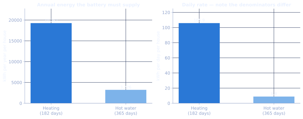
La cadena es: consumo específico → energía anual por vivienda → energía diaria en temporada → energía diaria de todo el conjunto. Calefacción y agua caliente se tratan por separado porque la calefacción funciona 182 días y el agua caliente los 365.
# Annual energy per house, split by end use
kwh_m2_heating   = SPECIFIC_KWH_M2_YR * FRAC_HEATING
kwh_m2_hot_water = SPECIFIC_KWH_M2_YR * FRAC_HOT_WATER

annual_heating   = kwh_m2_heating   * heated_area     # kWh/yr/house
annual_hot_water = kwh_m2_hot_water * heated_area     # kWh/yr/house

# Daily figures. Note the different denominators - this is the subtle bit.
daily_heating   = annual_heating   / HEATING_SEASON_DAYS   # only during the season
daily_hot_water = annual_hot_water / DAYS_PER_YEAR         # year round

daily_per_house  = daily_heating + daily_hot_water
daily_cluster    = daily_per_house * N_HOUSES

print(f"Heating    {kwh_m2_heating:6.2f} kWh/m2/yr -> {annual_heating:8,.0f} kWh/yr")
print(f"           spread over {HEATING_SEASON_DAYS} days -> {daily_heating:6.1f} kWh/day")
print(f"Hot water  {kwh_m2_hot_water:6.2f} kWh/m2/yr -> {annual_hot_water:8,.0f} kWh/yr")
print(f"           spread over {DAYS_PER_YEAR} days -> {daily_hot_water:6.1f} kWh/day")
print(f"\nTotal per house during the heating season: {daily_per_house:.1f} kWh/day")
print(f"Total for {N_HOUSES} houses:                     {daily_cluster:,.0f} kWh/day")

check("annual heating per house",  annual_heating,  19304.0, unit="kWh")
check("annual hot water per house", annual_hot_water, 3232.0, unit="kWh")
check("daily demand per house",     daily_per_house,   115.0, unit="kWh")
check("daily demand, cluster",      daily_cluster,    1955.0, unit="kWh")
Heating    121.41 kWh/m2/yr ->   19,267 kWh/yr
           spread over 182 days ->  105.9 kWh/day
Hot water   20.33 kWh/m2/yr ->    3,226 kWh/yr
           spread over 365 days ->    8.8 kWh/day

Total per house during the heating season: 114.7 kWh/day
Total for 17 houses:                     1,950 kWh/day
ok  annual heating per house           19,267.2 vs     19,304.0 kWh     0.19%
ok  annual hot water per house          3,226.3 vs      3,232.0 kWh     0.18%
ok  daily demand per house                114.7 vs        115.0 kWh     0.26%
ok  daily demand, cluster               1,949.9 vs      1,955.0 kWh     0.26%
fig, (ax1, ax2) = plt.subplots(1, 2, figsize=(11, 4.4))

# Left: where the annual energy goes
labels = ["Heating\n(182 days)", "Hot water\n(365 days)"]
annual = [annual_heating, annual_hot_water]
bars = ax1.bar(labels, annual, color=[PALETTE["accent"], PALETTE["accent_2"]], width=0.55)
for b, v in zip(bars, annual):
    ax1.text(b.get_x() + b.get_width()/2, v + 300, f"{v:,.0f}", ha="center", fontsize=10)
ax1.set_ylabel("kWh per year per house")
ax1.set_title("Annual energy the battery must supply")
ax1.set_ylim(0, max(annual) * 1.18)

# Right: the same energy expressed per day - the ratio inverts
daily = [daily_heating, daily_hot_water]
bars = ax2.bar(labels, daily, color=[PALETTE["accent"], PALETTE["accent_2"]], width=0.55)
for b, v in zip(bars, daily):
    ax2.text(b.get_x() + b.get_width()/2, v + 2, f"{v:.1f}", ha="center", fontsize=10)
ax2.set_ylabel("kWh per day per house")
ax2.set_title("Daily rate — note the denominators differ")
ax2.set_ylim(0, max(daily) * 1.18)

plt.tight_layout(); plt.show()

print(f"Heating is {annual_heating/annual_hot_water:.1f}x hot water over a year,")
print(f"but only {daily_heating/daily_hot_water:.1f}x on a winter day, because hot water is")
print("spread across all 365 days while heating is concentrated into 182.")
Heating is 6.0x hot water over a year,
but only 12.0x on a winter day, because hot water is
spread across all 365 days while heating is concentrated into 182.
Paso 2 — dimensionar el almacén
El almacén se dimensiona por calor sensible: sin cambio de fase, sin química, solo una masa de sólido que cambia de temperatura.
Una nota sobre unidades. El informe escribe la conversión como . Un kilovatio-hora son J, no —el resultado impreso ( J) es correcto, así que es una errata en el desarrollo y no un error en el diseño. La celda de abajo usa el factor correcto y llega al mismo número, que es la forma más barata posible de demostrarlo.
J_PER_KWH = 3.6e6      # not 3.6e3 - see the note above

energy_store_kwh = daily_cluster * AUTONOMY_DAYS
energy_store_J   = energy_store_kwh * J_PER_KWH

mass_s   = energy_store_J / (cp_eff * DELTA_T)
volume_s = mass_s / rho_eff

print(f"Energy to store ({AUTONOMY_DAYS} days autonomy): {energy_store_kwh:,.0f} kWh"
      f"  = {energy_store_J:.3e} J")
print(f"Ceramic mass required:                   {mass_s:,.0f} kg")
print(f"Bed volume required:                     {volume_s:,.1f} m3")

check("stored energy", energy_store_J, 1.408e10, unit="J")
check("ceramic mass",  mass_s,        38428.0,   unit="kg")
check("bed volume",    volume_s,         33.7,   unit="m3")
Energy to store (2 days autonomy): 3,900 kWh  = 1.404e+10 J
Ceramic mass required:                   38,334 kg
Bed volume required:                     33.6 m3
ok  stored energy                  14,039,599,503.0 vs 14,080,000,000.0 J       0.29%
ok  ceramic mass                       38,334.4 vs     38,428.0 kg      0.24%
ok  bed volume                             33.6 vs         33.7 m3      0.22%
Paso 3 — geometría
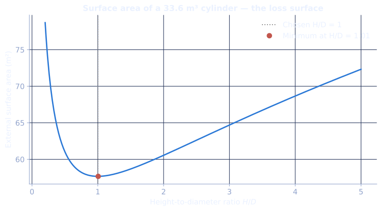
Se elige una relación altura-diámetro porque minimiza la superficie para un volumen dado, y la superficie es por donde se escapa el calor. Con :
La afirmación de que es óptimo merece comprobarse en lugar de darse por buena, así que la celda de abajo hace un barrido.
radius = (volume_s / (2 * np.pi)) ** (1/3)
height = 2 * radius

print(f"Cylinder: R = {radius:.2f} m, H = {height:.2f} m  (H/D = 1)")
check("radius", radius, 1.75, unit="m")
check("height", height, 3.50, unit="m")

def cylinder_area(vol, hd_ratio):
    '''Total external area (side + both ends) of a cylinder of given volume and H/D.'''
    r = (vol / (np.pi * 2 * hd_ratio)) ** (1/3)
    h = 2 * r * hd_ratio
    return 2*np.pi*r*h + 2*np.pi*r**2, r, h

hd = np.linspace(0.2, 5.0, 400)
areas = np.array([cylinder_area(volume_s, x)[0] for x in hd])
best = hd[np.argmin(areas)]

fig, ax = plt.subplots()
ax.plot(hd, areas, color=PALETTE["accent"], lw=2)
ax.axvline(1.0, color=PALETTE["faint"], ls=":", lw=1.4, label="Chosen H/D = 1")
ax.plot([best], [areas.min()], "o", color=PALETTE["warn"], ms=7,
        label=f"Minimum at H/D = {best:.2f}")
ax.set_xlabel("Height-to-diameter ratio $H/D$")
ax.set_ylabel("External surface area (m²)")
ax.set_title(f"Surface area of a {volume_s:.1f} m³ cylinder — the loss surface")
ax.legend(frameon=False)
plt.tight_layout(); plt.show()

a_chosen = cylinder_area(volume_s, 1.0)[0]
print(f"Area at H/D = 1: {a_chosen:.2f} m2")
print(f"True minimum:    {areas.min():.2f} m2 at H/D = {best:.2f}"
      f"  -> the chosen ratio is within {100*(a_chosen/areas.min()-1):.2f}% of optimal.")
print("\nH/D = 1 is not exactly optimal, but it is flat near the minimum and it is a")
print("far easier shape to build. That is a good engineering trade, and worth saying out loud.")
Cylinder: R = 1.75 m, H = 3.50 m  (H/D = 1)
ok  radius                                  1.7 vs          1.8 m       0.05%
ok  height                                  3.5 vs          3.5 m       0.05%
Area at H/D = 1: 57.67 m2
True minimum:    57.67 m2 at H/D = 1.01  -> the chosen ratio is within -0.00% of optimal.

H/D = 1 is not exactly optimal, but it is flat near the minimum and it is a
far easier shape to build. That is a good engineering trade, and worth saying out loud.
Paso 4 — potencia, no solo energía
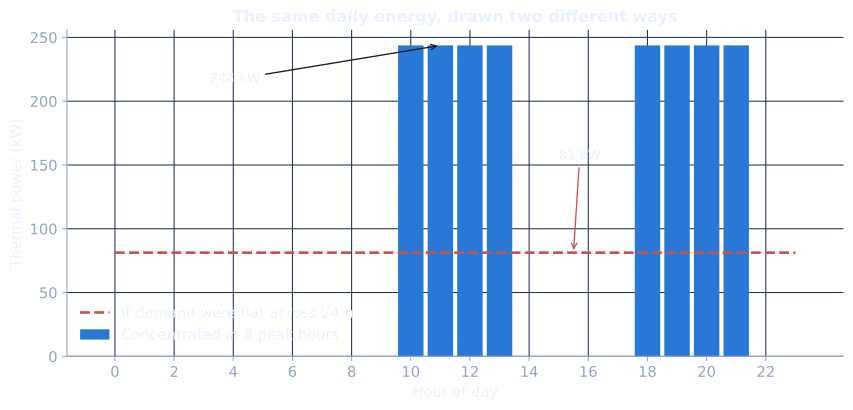
La energía dimensiona el montón. La potencia dimensiona las tuberías. Las tarifas españolas concentran la demanda residencial en dos franjas de horas punta —de 10:00 a 14:00 y de 18:00 a 22:00—, así que la energía diaria se extrae en unas 8 horas, no en 24:
PEAK_HOURS = 8

q_peak_kw = daily_cluster / PEAK_HOURS
q_avg_kw  = daily_cluster / 24

m_dot_peak = (q_peak_kw * 1000) / (CP_AIR * DELTA_T)
m_dot_avg  = (q_avg_kw  * 1000) / (CP_AIR * DELTA_T)

print(f"Peak thermal power   {q_peak_kw:7.1f} kW  -> air flow {m_dot_peak:.3f} kg/s")
print(f"Average over 24 h    {q_avg_kw:7.1f} kW  -> air flow {m_dot_avg:.3f} kg/s")
print(f"\nPeak is {q_peak_kw/q_avg_kw:.0f}x the daily average.")

check("peak power",    q_peak_kw,   244.4, unit="kW")
check("average power", q_avg_kw,     81.5, unit="kW")
check("peak air flow", m_dot_peak,  0.582, unit="kg/s")
check("avg air flow",  m_dot_avg,   0.194, unit="kg/s")
Peak thermal power     243.7 kW  -> air flow 0.580 kg/s
Average over 24 h       81.2 kW  -> air flow 0.193 kg/s

Peak is 3x the daily average.
ok  peak power                            243.7 vs        244.4 kW      0.27%
ok  average power                          81.2 vs         81.5 kW      0.31%
ok  peak air flow                           0.6 vs          0.6 kg/s    0.29%
ok  avg air flow                            0.2 vs          0.2 kg/s    0.29%
# What the day actually looks like: flat assumption vs the tariff windows.
hours = np.arange(24)
peak_mask = ((hours >= 10) & (hours < 14)) | ((hours >= 18) & (hours < 22))
profile_peaked = np.where(peak_mask, daily_cluster / PEAK_HOURS, 0.0)
profile_flat   = np.full(24, daily_cluster / 24)

fig, ax = plt.subplots(figsize=(9, 4.4))
ax.bar(hours, profile_peaked, width=0.86, color=PALETTE["accent"],
       label=f"Concentrated in {PEAK_HOURS} peak hours")
ax.plot(hours, profile_flat, color=PALETTE["warn"], lw=2, ls="--",
        label="If demand were flat across 24 h")
ax.set_xticks(hours[::2])
ax.set_xlabel("Hour of day")
ax.set_ylabel("Thermal power (kW)")
ax.set_title("The same daily energy, drawn two different ways")
ax.legend(frameon=False)
ax.annotate(f"{q_peak_kw:.0f} kW", xy=(11, q_peak_kw), xytext=(3.2, q_peak_kw*0.88),
            arrowprops=dict(arrowstyle="->", color=PALETTE["ink"], lw=1), fontsize=10)
ax.annotate(f"{q_avg_kw:.0f} kW", xy=(15.5, q_avg_kw), xytext=(15.0, q_avg_kw*1.9),
            arrowprops=dict(arrowstyle="->", color=PALETTE["warn"], lw=1),
            fontsize=10, color=PALETTE["warn"])
plt.tight_layout(); plt.show()

print("The pile is sized by the area under the curve; the fan and pipework are sized by its height.")
The pile is sized by the area under the curve; the fan and pipework are sized by its height.
4.3 Límites de funcionamiento
El informe enumera cuatro limitaciones en prosa. Cada una es un número al que este modelo puede ponerle tamaño, que es precisamente la razón de escribirlo como código.
¿Sobre qué hipótesis se sostiene el diseño?
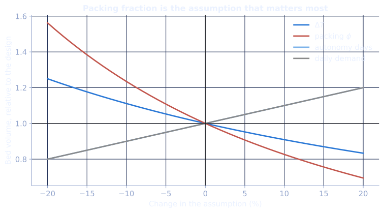
: la fracción de empaquetamiento aparece dos veces, una en la densidad efectiva y otra en el calor específico efectivo. Así que un error modesto en mueve el volumen de la batería mucho más que el mismo error en .
def bed_volume(delta_t=DELTA_T, phi=PACKING_PHI, days=AUTONOMY_DAYS,
               rho_s=RHO_S, cp_s=CP_S, daily_kwh=None):
    '''Bed volume in m3 for a given set of assumptions.'''
    daily_kwh = daily_cluster if daily_kwh is None else daily_kwh
    energy_J = daily_kwh * days * J_PER_KWH
    m = energy_J / ((phi * cp_s) * delta_t)
    return m / (phi * rho_s)

# One-at-a-time sensitivity: +/-20% on each assumption.
base = bed_volume()
factors = np.linspace(0.8, 1.2, 41)
curves = {
    r"$\Delta T$":            [bed_volume(delta_t=DELTA_T*f) for f in factors],
    r"packing $\phi$":        [bed_volume(phi=PACKING_PHI*f) for f in factors],
    "autonomy days":          [bed_volume(days=AUTONOMY_DAYS*f) for f in factors],
    "daily demand":           [bed_volume(daily_kwh=daily_cluster*f) for f in factors],
}

fig, ax = plt.subplots()
colors = [PALETTE["accent"], PALETTE["warn"], PALETTE["accent_2"], PALETTE["faint"]]
for (label, vals), c in zip(curves.items(), colors):
    ax.plot((factors - 1) * 100, np.array(vals) / base, lw=2, label=label, color=c)
ax.axhline(1, color=PALETTE["ink"], lw=0.8)
ax.axvline(0, color=PALETTE["ink"], lw=0.8)
ax.set_xlabel("Change in the assumption (%)")
ax.set_ylabel("Bed volume, relative to the design")
ax.set_title("Packing fraction is the assumption that matters most")
ax.legend(frameon=False)
plt.tight_layout(); plt.show()

lo, hi = bed_volume(phi=0.55), bed_volume(phi=0.65)
print(f"phi = 0.55 -> {lo:5.1f} m3     phi = 0.60 -> {base:5.1f} m3     phi = 0.65 -> {hi:5.1f} m3")
print(f"A +/-0.05 swing in a number nobody measured moves the battery by {(lo-hi):.1f} m3,")
print(f"which is {100*(lo-hi)/base:.0f}% of its volume.")
phi = 0.55 ->  40.0 m3     phi = 0.60 ->  33.6 m3     phi = 0.65 ->  28.7 m3
A +/-0.05 swing in a number nobody measured moves the battery by 11.4 m3,
which is 34% of its volume.
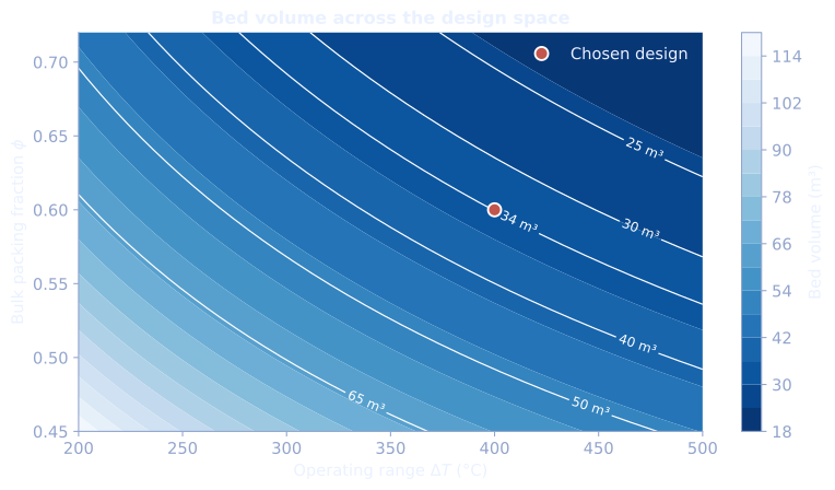
# Two-way sensitivity: the design space the battery lives in.
dt_vals  = np.linspace(200, 500, 140)
phi_vals = np.linspace(0.45, 0.72, 140)
DT, PHI = np.meshgrid(dt_vals, phi_vals)
VOL = np.vectorize(lambda d, p: bed_volume(delta_t=d, phi=p))(DT, PHI)

fig, ax = plt.subplots(figsize=(8.4, 4.8))
cf = ax.contourf(DT, PHI, VOL, levels=18, cmap="Blues_r")
cs = ax.contour(DT, PHI, VOL, levels=[25, 30, 33.7, 40, 50, 65],
                colors="white", linewidths=0.9)
ax.clabel(cs, fmt="%.0f m³", fontsize=9)
ax.plot([DELTA_T], [PACKING_PHI], "o", ms=9, color=PALETTE["warn"],
        markeredgecolor="white", markeredgewidth=1.4, label="Chosen design")
ax.set_xlabel(r"Operating range $\Delta T$ (°C)")
ax.set_ylabel(r"Bulk packing fraction $\phi$")
ax.set_title("Bed volume across the design space")
ax.legend(frameon=False, loc="upper right")
ax.grid(False)
fig.colorbar(cf, ax=ax, label="Bed volume (m³)")
plt.tight_layout(); plt.show()
El cuello de botella que el cálculo de energía no ve
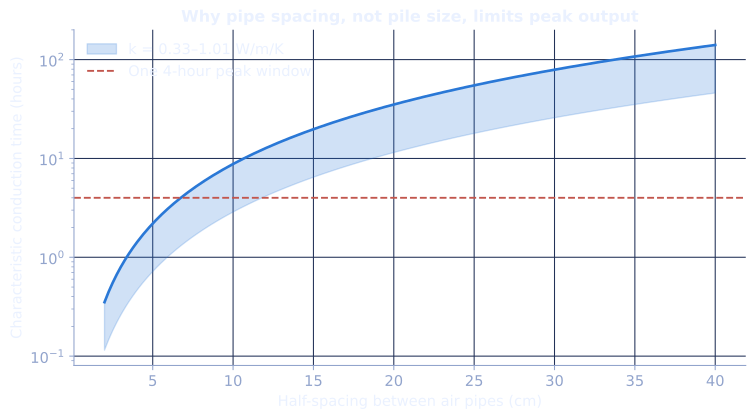
El almacén guarda energía suficiente. Si puede entregarla en punta es otra pregunta, y la gobierna la conductividad térmica de la cerámica, que es baja: 0,33–1,01 W/m/K.
El calor tiene que conducirse desde el grueso del lecho hasta los tubos de aire. El tiempo característico de conducción a lo largo de una distancia es
Ese es el problema: duplicar la separación entre tubos cuadruplica el tiempo.
k_lo, k_hi = K_S_RANGE
alpha_lo = k_lo / (rho_eff * cp_eff)     # m2/s, pessimistic
alpha_hi = k_hi / (rho_eff * cp_eff)     # m2/s, optimistic

spacing = np.linspace(0.02, 0.40, 300)   # half-distance from pipe to bed centre, m
t_lo = spacing**2 / alpha_hi / 3600      # hours, best case
t_hi = spacing**2 / alpha_lo / 3600      # hours, worst case

fig, ax = plt.subplots()
ax.fill_between(spacing*100, t_lo, t_hi, color=PALETTE["accent"], alpha=0.22,
                label=f"k = {k_lo}–{k_hi} W/m/K")
ax.plot(spacing*100, t_hi, color=PALETTE["accent"], lw=2)
ax.axhline(4, color=PALETTE["warn"], ls="--", lw=1.4,
           label="One 4-hour peak window")
ax.set_xlabel("Half-spacing between air pipes (cm)")
ax.set_ylabel("Characteristic conduction time (hours)")
ax.set_title("Why pipe spacing, not pile size, limits peak output")
ax.set_yscale("log")
ax.legend(frameon=False)
plt.tight_layout(); plt.show()

# The spacing at which conduction just keeps up with a 4-hour peak window.
L_ok = np.sqrt(alpha_lo * 4 * 3600)
print(f"Thermal diffusivity: {alpha_lo:.2e} to {alpha_hi:.2e} m2/s")
print(f"\nTo move heat within a single 4-hour peak window, worst-case conductivity needs")
print(f"pipes no more than about {L_ok*100:.0f} cm from any point in the bed.")
print(f"A {radius:.2f} m radius cylinder with no internal pipework has material {radius*100:.0f} cm")
print(f"from the wall — roughly {radius/L_ok:.0f}x too far. The pipe field is not optional,")
print("and the report is right to flag conduction as the binding constraint on peak delivery.")
Thermal diffusivity: 3.16e-07 to 9.68e-07 m2/s

To move heat within a single 4-hour peak window, worst-case conductivity needs
pipes no more than about 7 cm from any point in the bed.
A 1.75 m radius cylinder with no internal pipework has material 175 cm
from the wall — roughly 26x too far. The pipe field is not optional,
and the report is right to flag conduction as the binding constraint on peak delivery.
Los otros tres límites, cuantificados
- Vida en ciclos. La cerámica se ensayó durante más de 60 ciclos. Una temporada de calefacción son 182 días; a razón de un ciclo al día, aproximadamente, eso son tres temporadas de evidencia para un sistema pensado para durar décadas.
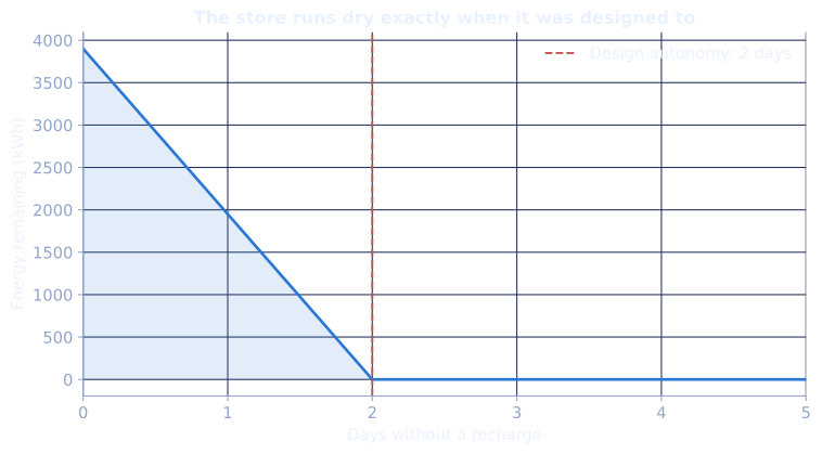
- Riesgo de rachas nubladas. Los dos días de autonomía se dimensionan con la nubosidad media de enero. Es una mediana, no un caso peor.
- Aire muerto. Con , el 40 % del cilindro es aire, que no almacena nada y además aísla la cerámica de los tubos.
run_hours = np.arange(0, 121, 1)
energy_left = np.clip(energy_store_kwh - (daily_cluster/24) * run_hours, 0, None)

fig, ax = plt.subplots()
ax.plot(run_hours/24, energy_left, color=PALETTE["accent"], lw=2)
ax.fill_between(run_hours/24, 0, energy_left, color=PALETTE["accent"], alpha=0.13)
ax.axvline(AUTONOMY_DAYS, color=PALETTE["warn"], ls="--", lw=1.4,
           label=f"Design autonomy: {AUTONOMY_DAYS} days")
ax.set_xlabel("Days without a recharge")
ax.set_ylabel("Energy remaining (kWh)")
ax.set_title("The store runs dry exactly when it was designed to")
ax.legend(frameon=False)
ax.set_xlim(0, 5)
plt.tight_layout(); plt.show()

for d in (3, 4, 5):
    extra = bed_volume(days=d)
    print(f"{d} days of autonomy would need {extra:5.1f} m3 "
          f"(+{100*(extra/base-1):3.0f}%), R = {(extra/(2*np.pi))**(1/3):.2f} m")
3 days of autonomy would need  50.4 m3 (+ 50%), R = 2.00 m
4 days of autonomy would need  67.3 m3 (+100%), R = 2.20 m
5 days of autonomy would need  84.1 m3 (+150%), R = 2.37 m
Lo que dice el modelo y el informe no podía decir
- La fracción de empaquetamiento es la hipótesis que sostiene la carga. Entra dos veces en el volumen, y es el único número del diseño sacado de una idealización de libro de texto («esferas empaquetadas al azar») en lugar de medido sobre la baldosa triturada real. Un error de ±0,05 mueve la batería en torno a una quinta parte de su volumen. Hay que medirla antes de construir nada.
- El corte a 150 °C equivale a unos 40 °C de rango sin usar. Lo fija el RITE, no la física, y el intercambiador cumple el requisito con mucho margen. Recuperar ese rango es la capacidad más barata disponible.
- no es el óptimo real, y no necesita serlo. La curva de superficie es plana cerca de su mínimo, así que la forma construible cuesta una fracción de un uno por ciento.
- El montón se dimensiona por energía; el sistema lo limita la conducción. Todos los resultados anteriores suponen que el calor llega a los tubos lo bastante rápido, y la difusividad dice que eso solo se cumple con un campo de tubos denso.
Reproducido de ENGF0004 Coursework 2, capítulo 4. El diseño, las fuentes y las decisiones de criterio son del trabajo; este notebook las vuelve a derivar para poder poner a prueba cada una.