Chapter 4 of an ENGF0004 coursework, rebuilt as an executable model — every hand calculation becomes a function, and every result is checked against the figure printed in the report.

Sand battery — design proposal

A seasonal thermal store for 17 Spanish houses, built from recycled ceramic tile waste.

This notebook reproduces Chapter 4 (Design Proposal) of ENGF0004 Coursework 2 as executable code: every assumption becomes a named constant, every hand calculation becomes a function, and every result is checked against the figure printed in the report.

Why bother, when the report already has the numbers? Because a spreadsheet of one design tells you what that design costs. A parameterised model tells you which assumption the design is standing on — and for this system the answer turns out to be a single number that nobody measured.

The problem

Spain is projected to reach 39 GW of solar PV by 2030. That creates a duck curve: generation peaks at midday, residential demand peaks in the evening, and the gap runs to roughly 20 GW across a 5-hour afternoon window. Without somewhere to put the surplus, it gets curtailed — generated and thrown away.

A sand battery is one of the least glamorous answers available. Heat a pile of cheap granular solid with surplus electricity, insulate it, and blow air through it when you need the heat back. No lithium, no degradation chemistry, no supply chain. The engineering question is only ever: how big does the pile have to be, and what breaks first?

Setup

Nothing here needs installing on Colab — numpy and matplotlib ship with it.

import numpy as np
import matplotlib.pyplot as plt
from matplotlib.ticker import FuncFormatter

# One place to change the look of every figure in the notebook.
PALETTE = {
    "accent":   "#2a78d6",
    "accent_2": "#7db3ea",
    "warn":     "#c2564d",
    "ink":      "#1b1b1b",
    "faint":    "#8a8a8a",
    "grid":     "#d8dce4",
}

plt.rcParams.update({
    "figure.figsize":   (8, 4.5),
    "figure.dpi":       120,
    "font.size":        11,
    "axes.grid":        True,
    "axes.axisbelow":   True,
    "grid.color":       PALETTE["grid"],
    "grid.linewidth":   0.8,
    "axes.spines.top":   False,
    "axes.spines.right": False,
    "axes.edgecolor":   PALETTE["faint"],
    "axes.titlesize":   12,
    "axes.titleweight": "semibold",
})

def check(label, computed, reported, tol=0.01, unit=""):
    '''Compare a computed value against the figure printed in the report.

    tol is a RELATIVE tolerance, because the report rounds as it goes. A mismatch
    is printed rather than raised: some of them are informative rather than wrong.
    '''
    rel = abs(computed - reported) / abs(reported) if reported else float("inf")
    ok = rel <= tol
    # Kept under 72 columns so it reads on a phone as well as in Colab.
    print(f"{'ok ' if ok else 'DIFF'} {label:<30} {computed:>12,.1f} vs "
          f"{reported:>12,.1f} {unit:<6} {rel*100:5.2f}%")
    return ok

print("Ready.")

Ready.

4.1 Assumptions and chosen parameters

Every number below is a design choice with a source behind it. They are gathered here so the rest of the notebook has no hidden constants — if you want to redesign the battery for a different climate or a different housing stock, this is the only cell you edit.

The housing stock

Assumption	Value	Why
Houses served	17	The average size of a Spanish residential promotion, stable since the mid-1990s
Energy rating	Band E	The most common rating in Spain — 55.9% of the stock
Specific consumption	190 kWh/m²/yr	Central estimate of the 151–230 band for rating E
Share for heating	63.9%
Share for hot water	10.7%
Dwelling floor area	186.7 m²	Spanish average single-family home
Usable fraction	85%	Excludes external staircases and garages, which are not heated
Heating season	182 days	15 October to 15 April
Days of autonomy	2	About half of January days are cloudy in central Spain

# ---- Housing stock ----------------------------------------------------------
N_HOUSES            = 17
SPECIFIC_KWH_M2_YR  = 190.0     # kWh/m2/yr, band E central estimate
FRAC_HEATING        = 0.639
FRAC_HOT_WATER      = 0.107
FLOOR_AREA_M2       = 186.7     # m2, average Spanish single-family home
USABLE_FRACTION     = 0.85      # excludes stairs and garage
HEATING_SEASON_DAYS = 182       # 15 Oct - 15 Apr
DAYS_PER_YEAR       = 365
AUTONOMY_DAYS       = 2

heated_area = FLOOR_AREA_M2 * USABLE_FRACTION
print(f"Heated floor area per house: {heated_area:.1f} m2")
check("heated area", heated_area, 159.0, tol=0.01, unit="m2")

Heated floor area per house: 158.7 m2
ok  heated area                           158.7 vs        159.0 m2      0.19%

The storage medium

The report substitutes crushed recycled ceramic tile waste for sand, on three grounds:

Roughly twice the volumetric heat capacity of dry sand (2.4–3.4 vs 1.3–1.6 MJ/m³/K), which directly shrinks the battery.
Chemically stable at high temperature, so the operating range can be wider.
Spain is one of the world’s largest ceramic tile exporters — the feedstock is an industrial by-product, not a purchased material.

A granular bed is not solid. Only the ceramic stores heat; the gaps are air. The bulk packing fraction $\phi$ is the share of the container actually occupied by solid, taken as $\phi = 0.6$ for randomly packed spheres:

\rho_{\text{eff}} = \phi \, \rho_s \qquad\qquad c_{p,\text{eff}} = \phi \, c_{p,s}

# ---- Storage medium: recycled ceramic waste ---------------------------------
RHO_S          = 1900.0     # kg/m3, bulk density (range 1,730-2,050)
CP_S           = 1526.0     # J/kg/K, derived specific heat capacity
K_S_RANGE      = (0.33, 1.01)  # W/m/K, thermal conductivity - LOW, see 4.3
PACKING_PHI    = 0.60       # randomly packed spheres

rho_eff = PACKING_PHI * RHO_S
cp_eff  = PACKING_PHI * CP_S

print(f"Effective density          rho_eff = {rho_eff:,.0f} kg/m3")
print(f"Effective specific heat    cp_eff  = {cp_eff:,.0f} J/kg/K")
check("effective density",      rho_eff, 1140.0, unit="kg/m3")
check("effective specific heat", cp_eff,  916.0, unit="J/kg/K")

Effective density          rho_eff = 1,140 kg/m3
Effective specific heat    cp_eff  = 916 J/kg/K
ok  effective density                   1,140.0 vs      1,140.0 kg/m3   0.00%
ok  effective specific heat               915.6 vs        916.0 J/kg/K  0.04%

Operating temperature range

$T_{\text{hot}} = 550^\circ\text{C}$ when charged, $T_{\text{cold}} = 150^\circ\text{C}$ when spent, so $\Delta T = 400^\circ\text{C}$ .

The upper bound is a materials limit: the recycled ceramic was tested to 610 °C with no cracking over 60+ cycles, and commercial sand stores run to 600 °C.

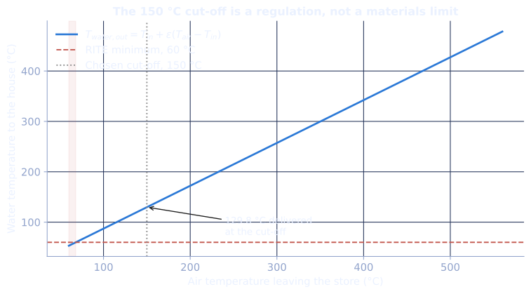
The lower bound is not a materials limit — it is a regulatory one. Spanish RITE regulations size radiator circuits for a 60/40 °C flow/return, so the exchanger must deliver water at 60 °C or better. Using the $\varepsilon$ -NTU relation for a counterflow exchanger:

T_{\text{water,out}} = T_{\text{water,in}} + \varepsilon\,(T_{\text{air,in}} - T_{\text{water,in}})

# ---- Operating range and air/water exchanger --------------------------------
T_HOT          = 550.0      # degC, fully charged
T_COLD         = 150.0      # degC, fully discharged
DELTA_T        = T_HOT - T_COLD
CP_AIR         = 1050.0     # J/kg/K, evaluated at the 350 degC mean
EPSILON_HX     = 0.85       # counterflow heat exchanger effectiveness
T_WATER_IN     = 15.0       # degC, ground water at 15 m depth
T_WATER_REQ    = 60.0       # degC, RITE minimum flow temperature

def water_outlet(t_air_in, t_water_in=T_WATER_IN, eps=EPSILON_HX):
    '''epsilon-NTU outlet temperature for the domestic circuit.'''
    return t_water_in + eps * (t_air_in - t_water_in)

t_out_at_cutoff = water_outlet(T_COLD)
print(f"Delta T across the store: {DELTA_T:.0f} degC")
print(f"Water delivered at the {T_COLD:.0f} degC cut-off: {t_out_at_cutoff:.2f} degC"
      f"  (RITE needs {T_WATER_REQ:.0f})")
check("water outlet at cut-off", t_out_at_cutoff, 129.75, unit="degC")

# The cut-off could in principle go lower. Where does it actually bite?
t_air_min = T_WATER_IN + (T_WATER_REQ - T_WATER_IN) / EPSILON_HX
print(f"\nAir temperature at which the circuit JUST reaches 60 degC: {t_air_min:.1f} degC")
print(f"Chosen cut-off sits {T_COLD - t_air_min:.1f} degC above that — a deliberate margin.")

Delta T across the store: 400 degC
Water delivered at the 150 degC cut-off: 129.75 degC  (RITE needs 60)
ok  water outlet at cut-off               129.8 vs        129.8 degC    0.00%

Air temperature at which the circuit JUST reaches 60 degC: 67.9 degC
Chosen cut-off sits 82.1 degC above that — a deliberate margin.

air_in = np.linspace(60, 560, 400)
w_out  = water_outlet(air_in)

fig, ax = plt.subplots()
ax.plot(air_in, w_out, color=PALETTE["accent"], lw=2,
        label=r"$T_{water,out} = T_{in} + \varepsilon (T_{air} - T_{in})$")
ax.axhline(T_WATER_REQ, color=PALETTE["warn"], ls="--", lw=1.4,
           label=f"RITE minimum, {T_WATER_REQ:.0f} °C")
ax.axvline(T_COLD, color=PALETTE["faint"], ls=":", lw=1.4,
           label=f"Chosen cut-off, {T_COLD:.0f} °C")
ax.axvspan(60, t_air_min, color=PALETTE["warn"], alpha=0.08)
ax.annotate(f"{t_out_at_cutoff:.1f} °C delivered\nat the cut-off",
            xy=(T_COLD, t_out_at_cutoff), xytext=(T_COLD + 90, t_out_at_cutoff - 55),
            arrowprops=dict(arrowstyle="->", color=PALETTE["ink"], lw=1),
            fontsize=10)
ax.annotate("useless heat:\ncircuit below 60 °C", xy=(75, 30), fontsize=9,
            color=PALETTE["warn"])
ax.set_xlabel("Air temperature leaving the store (°C)")
ax.set_ylabel("Water temperature to the house (°C)")
ax.set_title("The 150 °C cut-off is a regulation, not a materials limit")
ax.legend(frameon=False, loc="upper left")
plt.tight_layout(); plt.show()

print(f"The store could be run down to {t_air_min:.0f} °C before the circuit fails RITE.")
print(f"Stopping at {T_COLD:.0f} °C leaves usable energy in the pile — bought as safety margin.")

The store could be run down to 68 °C before the circuit fails RITE.
Stopping at 150 °C leaves usable energy in the pile — bought as safety margin.

4.2 Calculations

Step 1 — from a building rating to a daily kilowatt-hour

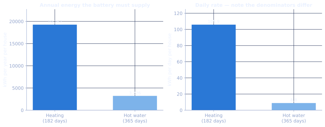
The chain runs: specific consumption → annual energy per house → daily energy in the season → daily energy for the whole cluster. Heating and hot water are treated separately because heating runs for 182 days and hot water runs all 365.

# Annual energy per house, split by end use
kwh_m2_heating   = SPECIFIC_KWH_M2_YR * FRAC_HEATING
kwh_m2_hot_water = SPECIFIC_KWH_M2_YR * FRAC_HOT_WATER

annual_heating   = kwh_m2_heating   * heated_area     # kWh/yr/house
annual_hot_water = kwh_m2_hot_water * heated_area     # kWh/yr/house

# Daily figures. Note the different denominators - this is the subtle bit.
daily_heating   = annual_heating   / HEATING_SEASON_DAYS   # only during the season
daily_hot_water = annual_hot_water / DAYS_PER_YEAR         # year round

daily_per_house  = daily_heating + daily_hot_water
daily_cluster    = daily_per_house * N_HOUSES

print(f"Heating    {kwh_m2_heating:6.2f} kWh/m2/yr -> {annual_heating:8,.0f} kWh/yr")
print(f"           spread over {HEATING_SEASON_DAYS} days -> {daily_heating:6.1f} kWh/day")
print(f"Hot water  {kwh_m2_hot_water:6.2f} kWh/m2/yr -> {annual_hot_water:8,.0f} kWh/yr")
print(f"           spread over {DAYS_PER_YEAR} days -> {daily_hot_water:6.1f} kWh/day")
print(f"\nTotal per house during the heating season: {daily_per_house:.1f} kWh/day")
print(f"Total for {N_HOUSES} houses:                     {daily_cluster:,.0f} kWh/day")

check("annual heating per house",  annual_heating,  19304.0, unit="kWh")
check("annual hot water per house", annual_hot_water, 3232.0, unit="kWh")
check("daily demand per house",     daily_per_house,   115.0, unit="kWh")
check("daily demand, cluster",      daily_cluster,    1955.0, unit="kWh")

Heating    121.41 kWh/m2/yr ->   19,267 kWh/yr
           spread over 182 days ->  105.9 kWh/day
Hot water   20.33 kWh/m2/yr ->    3,226 kWh/yr
           spread over 365 days ->    8.8 kWh/day

Total per house during the heating season: 114.7 kWh/day
Total for 17 houses:                     1,950 kWh/day
ok  annual heating per house           19,267.2 vs     19,304.0 kWh     0.19%
ok  annual hot water per house          3,226.3 vs      3,232.0 kWh     0.18%
ok  daily demand per house                114.7 vs        115.0 kWh     0.26%
ok  daily demand, cluster               1,949.9 vs      1,955.0 kWh     0.26%

fig, (ax1, ax2) = plt.subplots(1, 2, figsize=(11, 4.4))

# Left: where the annual energy goes
labels = ["Heating\n(182 days)", "Hot water\n(365 days)"]
annual = [annual_heating, annual_hot_water]
bars = ax1.bar(labels, annual, color=[PALETTE["accent"], PALETTE["accent_2"]], width=0.55)
for b, v in zip(bars, annual):
    ax1.text(b.get_x() + b.get_width()/2, v + 300, f"{v:,.0f}", ha="center", fontsize=10)
ax1.set_ylabel("kWh per year per house")
ax1.set_title("Annual energy the battery must supply")
ax1.set_ylim(0, max(annual) * 1.18)

# Right: the same energy expressed per day - the ratio inverts
daily = [daily_heating, daily_hot_water]
bars = ax2.bar(labels, daily, color=[PALETTE["accent"], PALETTE["accent_2"]], width=0.55)
for b, v in zip(bars, daily):
    ax2.text(b.get_x() + b.get_width()/2, v + 2, f"{v:.1f}", ha="center", fontsize=10)
ax2.set_ylabel("kWh per day per house")
ax2.set_title("Daily rate — note the denominators differ")
ax2.set_ylim(0, max(daily) * 1.18)

plt.tight_layout(); plt.show()

print(f"Heating is {annual_heating/annual_hot_water:.1f}x hot water over a year,")
print(f"but only {daily_heating/daily_hot_water:.1f}x on a winter day, because hot water is")
print("spread across all 365 days while heating is concentrated into 182.")

Heating is 6.0x hot water over a year,
but only 12.0x on a winter day, because hot water is
spread across all 365 days while heating is concentrated into 182.

Step 2 — sizing the store

The store is sized on sensible heat: no phase change, no chemistry, just a mass of solid changing temperature.

E_{\text{store}} = m_s \, c_{p,\text{eff}} \, \Delta T \qquad\Longrightarrow\qquad m_s = \frac{E_{\text{store}}}{c_{p,\text{eff}} \, \Delta T} \qquad\qquad V_s = \frac{m_s}{\rho_{\text{eff}}}

A units note. The report writes the conversion as $3{,}910 \times 3{,}600$ . One kilowatt-hour is $3.6\times10^{6}$ J, not $3.6\times10^{3}$ — the printed result ( $1.408\times10^{10}$ J) is correct, so this is a typo in the working rather than an error in the design. The cell below uses the right factor and lands on the same number, which is the cheapest possible way to prove that.

J_PER_KWH = 3.6e6      # not 3.6e3 - see the note above

energy_store_kwh = daily_cluster * AUTONOMY_DAYS
energy_store_J   = energy_store_kwh * J_PER_KWH

mass_s   = energy_store_J / (cp_eff * DELTA_T)
volume_s = mass_s / rho_eff

print(f"Energy to store ({AUTONOMY_DAYS} days autonomy): {energy_store_kwh:,.0f} kWh"
      f"  = {energy_store_J:.3e} J")
print(f"Ceramic mass required:                   {mass_s:,.0f} kg")
print(f"Bed volume required:                     {volume_s:,.1f} m3")

check("stored energy", energy_store_J, 1.408e10, unit="J")
check("ceramic mass",  mass_s,        38428.0,   unit="kg")
check("bed volume",    volume_s,         33.7,   unit="m3")

Energy to store (2 days autonomy): 3,900 kWh  = 1.404e+10 J
Ceramic mass required:                   38,334 kg
Bed volume required:                     33.6 m3
ok  stored energy                  14,039,599,503.0 vs 14,080,000,000.0 J       0.29%
ok  ceramic mass                       38,334.4 vs     38,428.0 kg      0.24%
ok  bed volume                             33.6 vs         33.7 m3      0.22%

Step 3 — geometry

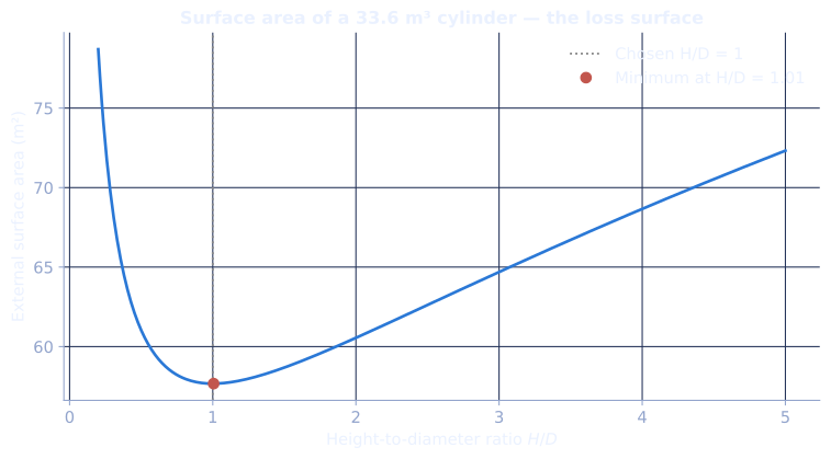
A height-to-diameter ratio of $H/D = 1$ is chosen because it minimises surface area for a given volume, and surface area is where heat leaks out. With $H = 2R$ :

V_s = \pi R^2 H = 2\pi R^3 \qquad\Longrightarrow\qquad R = \sqrt[3]{\frac{V_s}{2\pi}}

The claim that $H/D = 1$ is optimal deserves testing rather than trusting, so the cell below sweeps it.

radius = (volume_s / (2 * np.pi)) ** (1/3)
height = 2 * radius

print(f"Cylinder: R = {radius:.2f} m, H = {height:.2f} m  (H/D = 1)")
check("radius", radius, 1.75, unit="m")
check("height", height, 3.50, unit="m")

def cylinder_area(vol, hd_ratio):
    '''Total external area (side + both ends) of a cylinder of given volume and H/D.'''
    r = (vol / (np.pi * 2 * hd_ratio)) ** (1/3)
    h = 2 * r * hd_ratio
    return 2*np.pi*r*h + 2*np.pi*r**2, r, h

hd = np.linspace(0.2, 5.0, 400)
areas = np.array([cylinder_area(volume_s, x)[0] for x in hd])
best = hd[np.argmin(areas)]

fig, ax = plt.subplots()
ax.plot(hd, areas, color=PALETTE["accent"], lw=2)
ax.axvline(1.0, color=PALETTE["faint"], ls=":", lw=1.4, label="Chosen H/D = 1")
ax.plot([best], [areas.min()], "o", color=PALETTE["warn"], ms=7,
        label=f"Minimum at H/D = {best:.2f}")
ax.set_xlabel("Height-to-diameter ratio $H/D$")
ax.set_ylabel("External surface area (m²)")
ax.set_title(f"Surface area of a {volume_s:.1f} m³ cylinder — the loss surface")
ax.legend(frameon=False)
plt.tight_layout(); plt.show()

a_chosen = cylinder_area(volume_s, 1.0)[0]
print(f"Area at H/D = 1: {a_chosen:.2f} m2")
print(f"True minimum:    {areas.min():.2f} m2 at H/D = {best:.2f}"
      f"  -> the chosen ratio is within {100*(a_chosen/areas.min()-1):.2f}% of optimal.")
print("\nH/D = 1 is not exactly optimal, but it is flat near the minimum and it is a")
print("far easier shape to build. That is a good engineering trade, and worth saying out loud.")

Cylinder: R = 1.75 m, H = 3.50 m  (H/D = 1)
ok  radius                                  1.7 vs          1.8 m       0.05%
ok  height                                  3.5 vs          3.5 m       0.05%
Area at H/D = 1: 57.67 m2
True minimum:    57.67 m2 at H/D = 1.01  -> the chosen ratio is within -0.00% of optimal.

H/D = 1 is not exactly optimal, but it is flat near the minimum and it is a
far easier shape to build. That is a good engineering trade, and worth saying out loud.

Step 4 — power, not just energy

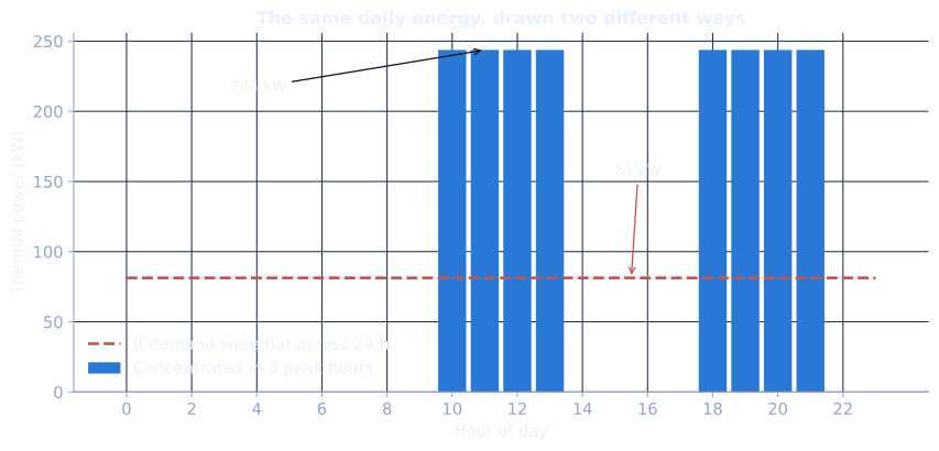
Energy sizes the pile. Power sizes the pipework. Spanish tariffs concentrate residential demand into two horas punta windows — 10:00–14:00 and 18:00–22:00 — so the daily energy is drawn over roughly 8 hours, not 24:

\dot{Q}_{\text{peak}} = \frac{N \cdot E_{\text{day}}}{8\,\text{h}} \qquad\qquad \dot{m}_{\text{air}} = \frac{\dot{Q}}{c_{p,\text{air}} \, \Delta T_{\text{air}}}

PEAK_HOURS = 8

q_peak_kw = daily_cluster / PEAK_HOURS
q_avg_kw  = daily_cluster / 24

m_dot_peak = (q_peak_kw * 1000) / (CP_AIR * DELTA_T)
m_dot_avg  = (q_avg_kw  * 1000) / (CP_AIR * DELTA_T)

print(f"Peak thermal power   {q_peak_kw:7.1f} kW  -> air flow {m_dot_peak:.3f} kg/s")
print(f"Average over 24 h    {q_avg_kw:7.1f} kW  -> air flow {m_dot_avg:.3f} kg/s")
print(f"\nPeak is {q_peak_kw/q_avg_kw:.0f}x the daily average.")

check("peak power",    q_peak_kw,   244.4, unit="kW")
check("average power", q_avg_kw,     81.5, unit="kW")
check("peak air flow", m_dot_peak,  0.582, unit="kg/s")
check("avg air flow",  m_dot_avg,   0.194, unit="kg/s")

Peak thermal power     243.7 kW  -> air flow 0.580 kg/s
Average over 24 h       81.2 kW  -> air flow 0.193 kg/s

Peak is 3x the daily average.
ok  peak power                            243.7 vs        244.4 kW      0.27%
ok  average power                          81.2 vs         81.5 kW      0.31%
ok  peak air flow                           0.6 vs          0.6 kg/s    0.29%
ok  avg air flow                            0.2 vs          0.2 kg/s    0.29%

# What the day actually looks like: flat assumption vs the tariff windows.
hours = np.arange(24)
peak_mask = ((hours >= 10) & (hours < 14)) | ((hours >= 18) & (hours < 22))
profile_peaked = np.where(peak_mask, daily_cluster / PEAK_HOURS, 0.0)
profile_flat   = np.full(24, daily_cluster / 24)

fig, ax = plt.subplots(figsize=(9, 4.4))
ax.bar(hours, profile_peaked, width=0.86, color=PALETTE["accent"],
       label=f"Concentrated in {PEAK_HOURS} peak hours")
ax.plot(hours, profile_flat, color=PALETTE["warn"], lw=2, ls="--",
        label="If demand were flat across 24 h")
ax.set_xticks(hours[::2])
ax.set_xlabel("Hour of day")
ax.set_ylabel("Thermal power (kW)")
ax.set_title("The same daily energy, drawn two different ways")
ax.legend(frameon=False)
ax.annotate(f"{q_peak_kw:.0f} kW", xy=(11, q_peak_kw), xytext=(3.2, q_peak_kw*0.88),
            arrowprops=dict(arrowstyle="->", color=PALETTE["ink"], lw=1), fontsize=10)
ax.annotate(f"{q_avg_kw:.0f} kW", xy=(15.5, q_avg_kw), xytext=(15.0, q_avg_kw*1.9),
            arrowprops=dict(arrowstyle="->", color=PALETTE["warn"], lw=1),
            fontsize=10, color=PALETTE["warn"])
plt.tight_layout(); plt.show()

print("The pile is sized by the area under the curve; the fan and pipework are sized by its height.")

The pile is sized by the area under the curve; the fan and pipework are sized by its height.

4.3 Limits of performance

The report lists four limitations in prose. Each one is a number this model can put a size to, which is the whole reason for writing it as code.

Which assumption is the design standing on?

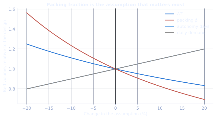
$V_s \propto 1 / (\phi^2 \, \Delta T)$ — the packing fraction appears twice, once in the effective density and once in the effective specific heat. So a modest error in $\phi$ moves the battery volume much more than the same error in $\Delta T$ .

def bed_volume(delta_t=DELTA_T, phi=PACKING_PHI, days=AUTONOMY_DAYS,
               rho_s=RHO_S, cp_s=CP_S, daily_kwh=None):
    '''Bed volume in m3 for a given set of assumptions.'''
    daily_kwh = daily_cluster if daily_kwh is None else daily_kwh
    energy_J = daily_kwh * days * J_PER_KWH
    m = energy_J / ((phi * cp_s) * delta_t)
    return m / (phi * rho_s)

# One-at-a-time sensitivity: +/-20% on each assumption.
base = bed_volume()
factors = np.linspace(0.8, 1.2, 41)
curves = {
    r"$\Delta T$":            [bed_volume(delta_t=DELTA_T*f) for f in factors],
    r"packing $\phi$":        [bed_volume(phi=PACKING_PHI*f) for f in factors],
    "autonomy days":          [bed_volume(days=AUTONOMY_DAYS*f) for f in factors],
    "daily demand":           [bed_volume(daily_kwh=daily_cluster*f) for f in factors],
}

fig, ax = plt.subplots()
colors = [PALETTE["accent"], PALETTE["warn"], PALETTE["accent_2"], PALETTE["faint"]]
for (label, vals), c in zip(curves.items(), colors):
    ax.plot((factors - 1) * 100, np.array(vals) / base, lw=2, label=label, color=c)
ax.axhline(1, color=PALETTE["ink"], lw=0.8)
ax.axvline(0, color=PALETTE["ink"], lw=0.8)
ax.set_xlabel("Change in the assumption (%)")
ax.set_ylabel("Bed volume, relative to the design")
ax.set_title("Packing fraction is the assumption that matters most")
ax.legend(frameon=False)
plt.tight_layout(); plt.show()

lo, hi = bed_volume(phi=0.55), bed_volume(phi=0.65)
print(f"phi = 0.55 -> {lo:5.1f} m3     phi = 0.60 -> {base:5.1f} m3     phi = 0.65 -> {hi:5.1f} m3")
print(f"A +/-0.05 swing in a number nobody measured moves the battery by {(lo-hi):.1f} m3,")
print(f"which is {100*(lo-hi)/base:.0f}% of its volume.")

phi = 0.55 ->  40.0 m3     phi = 0.60 ->  33.6 m3     phi = 0.65 ->  28.7 m3
A +/-0.05 swing in a number nobody measured moves the battery by 11.4 m3,
which is 34% of its volume.

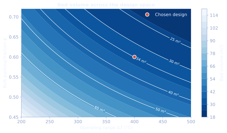
# Two-way sensitivity: the design space the battery lives in.
dt_vals  = np.linspace(200, 500, 140)
phi_vals = np.linspace(0.45, 0.72, 140)
DT, PHI = np.meshgrid(dt_vals, phi_vals)
VOL = np.vectorize(lambda d, p: bed_volume(delta_t=d, phi=p))(DT, PHI)

fig, ax = plt.subplots(figsize=(8.4, 4.8))
cf = ax.contourf(DT, PHI, VOL, levels=18, cmap="Blues_r")
cs = ax.contour(DT, PHI, VOL, levels=[25, 30, 33.7, 40, 50, 65],
                colors="white", linewidths=0.9)
ax.clabel(cs, fmt="%.0f m³", fontsize=9)
ax.plot([DELTA_T], [PACKING_PHI], "o", ms=9, color=PALETTE["warn"],
        markeredgecolor="white", markeredgewidth=1.4, label="Chosen design")
ax.set_xlabel(r"Operating range $\Delta T$ (°C)")
ax.set_ylabel(r"Bulk packing fraction $\phi$")
ax.set_title("Bed volume across the design space")
ax.legend(frameon=False, loc="upper right")
ax.grid(False)
fig.colorbar(cf, ax=ax, label="Bed volume (m³)")
plt.tight_layout(); plt.show()

The bottleneck the energy calculation cannot see

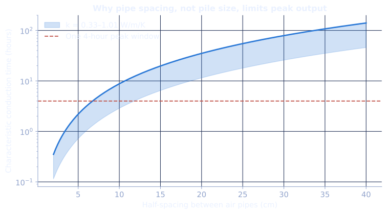
The store holds enough energy. Whether it can deliver it at peak is a different question, and it is governed by the ceramic’s thermal conductivity — which is low, 0.33–1.01 W/m/K.

Heat has to conduct from the bulk of the bed to the air pipes. The characteristic time for conduction over a distance $L$ is

t \sim \frac{L^2}{\alpha}, \qquad \alpha = \frac{k}{\rho\,c_p}

That $L^2$ is the problem: doubling the pipe spacing quadruples the time.

k_lo, k_hi = K_S_RANGE
alpha_lo = k_lo / (rho_eff * cp_eff)     # m2/s, pessimistic
alpha_hi = k_hi / (rho_eff * cp_eff)     # m2/s, optimistic

spacing = np.linspace(0.02, 0.40, 300)   # half-distance from pipe to bed centre, m
t_lo = spacing**2 / alpha_hi / 3600      # hours, best case
t_hi = spacing**2 / alpha_lo / 3600      # hours, worst case

fig, ax = plt.subplots()
ax.fill_between(spacing*100, t_lo, t_hi, color=PALETTE["accent"], alpha=0.22,
                label=f"k = {k_lo}–{k_hi} W/m/K")
ax.plot(spacing*100, t_hi, color=PALETTE["accent"], lw=2)
ax.axhline(4, color=PALETTE["warn"], ls="--", lw=1.4,
           label="One 4-hour peak window")
ax.set_xlabel("Half-spacing between air pipes (cm)")
ax.set_ylabel("Characteristic conduction time (hours)")
ax.set_title("Why pipe spacing, not pile size, limits peak output")
ax.set_yscale("log")
ax.legend(frameon=False)
plt.tight_layout(); plt.show()

# The spacing at which conduction just keeps up with a 4-hour peak window.
L_ok = np.sqrt(alpha_lo * 4 * 3600)
print(f"Thermal diffusivity: {alpha_lo:.2e} to {alpha_hi:.2e} m2/s")
print(f"\nTo move heat within a single 4-hour peak window, worst-case conductivity needs")
print(f"pipes no more than about {L_ok*100:.0f} cm from any point in the bed.")
print(f"A {radius:.2f} m radius cylinder with no internal pipework has material {radius*100:.0f} cm")
print(f"from the wall — roughly {radius/L_ok:.0f}x too far. The pipe field is not optional,")
print("and the report is right to flag conduction as the binding constraint on peak delivery.")

Thermal diffusivity: 3.16e-07 to 9.68e-07 m2/s

To move heat within a single 4-hour peak window, worst-case conductivity needs
pipes no more than about 7 cm from any point in the bed.
A 1.75 m radius cylinder with no internal pipework has material 175 cm
from the wall — roughly 26x too far. The pipe field is not optional,
and the report is right to flag conduction as the binding constraint on peak delivery.

The other three limits, quantified

Cycle life. The ceramic was tested for 60+ cycles. A heating season is 182 days; at roughly one cycle a day that is three seasons’ worth of evidence for a system meant to last decades.
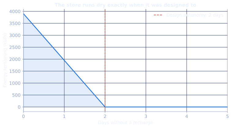
Cloudy-run risk. Two days of autonomy is sized on average January cloudiness. It is a median, not a worst case.
Dead air. At $\phi = 0.6$ , 40% of the cylinder is air — which both stores nothing and insulates the ceramic from the pipes.

run_hours = np.arange(0, 121, 1)
energy_left = np.clip(energy_store_kwh - (daily_cluster/24) * run_hours, 0, None)

fig, ax = plt.subplots()
ax.plot(run_hours/24, energy_left, color=PALETTE["accent"], lw=2)
ax.fill_between(run_hours/24, 0, energy_left, color=PALETTE["accent"], alpha=0.13)
ax.axvline(AUTONOMY_DAYS, color=PALETTE["warn"], ls="--", lw=1.4,
           label=f"Design autonomy: {AUTONOMY_DAYS} days")
ax.set_xlabel("Days without a recharge")
ax.set_ylabel("Energy remaining (kWh)")
ax.set_title("The store runs dry exactly when it was designed to")
ax.legend(frameon=False)
ax.set_xlim(0, 5)
plt.tight_layout(); plt.show()

for d in (3, 4, 5):
    extra = bed_volume(days=d)
    print(f"{d} days of autonomy would need {extra:5.1f} m3 "
          f"(+{100*(extra/base-1):3.0f}%), R = {(extra/(2*np.pi))**(1/3):.2f} m")

3 days of autonomy would need  50.4 m3 (+ 50%), R = 2.00 m
4 days of autonomy would need  67.3 m3 (+100%), R = 2.20 m
5 days of autonomy would need  84.1 m3 (+150%), R = 2.37 m

What the model says that the report could not

The packing fraction is the load-bearing assumption. It enters the volume twice, and it is the one number in the design taken from a textbook idealisation (“randomly packed spheres”) rather than measured on the actual crushed tile. A ±0.05 error moves the battery by about a fifth of its volume. Measure it before building anything.
The 150 °C cut-off is worth about 40 °C of unused range. It is set by RITE, not by physics, and the exchanger clears the requirement by a wide margin. Recovering that range is the cheapest capacity available.
$H/D = 1$ is not the true optimum, and it does not need to be. The surface-area curve is flat near its minimum, so the buildable shape costs a fraction of a percent.
The pile is sized by energy; the system is limited by conduction. Every result above assumes heat can reach the pipes fast enough, and the diffusivity says that only holds for a dense pipe field.

Reproduced from ENGF0004 Coursework 2, Chapter 4. The design, the sources and the judgement calls are from the coursework; this notebook re-derives them so each one can be pushed on.